
Many years ago, towards the end of the Cold War, I was an analyst at a defense research establishment. I built, maintained, and ran discrete event simulation models of large-scale air warfare, effectively modeling the Third World War in the airspace over Europe.
These were large and complex models. My Master’s thesis was on embedding a non-linear resource allocation model for prioritization between different possible mission types given the current state of the simulated combat inside one of these models. This represented the decisions of a human air commander, while an actual Air Vice Marshal was looking over my shoulder sharing helpful and specific advice like “Hey! I wouldn’t have done that!” (Later, I also found out that having one’s Master’s thesis classified for reasons of national security is somewhat inconvenient for future career reference.)
Our task was to give recommendations to senior decision-makers on important choices that could involve billions of dollars in peacetime cost and would have life-or-death consequences if the Cold War had turned hot. Moreover, some of these choices had their proponents and detractors with strong and vocal opinions, and with varying numbers of stars on their shoulderpads. No pressure whatsoever.
We were running these simulations on a cluster of VAXstations. These were powerful workstations for their time, providing about 11 MFLOPS from a single CPU core.
For comparison, a 2016 Apple Watch gave about 1 200 MFLOPS from its quadcore ARM Qualcomm CPU.
Quite literally, we were running large, complex high-stakes simulations on hardware with less than 1 % of the computing power that a ten-year-old wristwatch has today.
Suppose, for the sake of the argument, that there is a thing to evaluate. It could be a device, a tactic, a training program – whatever. Suppose also that the main outcome metric is a probability, e.g., of “winning” (whatever that means in the relevant scenario). As always, the proponents of the thing claim that it is the greatest thing since the invention of gunpowder, while the detractors think it could lose us the whole war in an afternoon.
So we load up the simulation, run it… and blue “won”! Success!
To which the Chief Scientist, who has seen things before, sagely comments, “That is just a single replication. Is it statistically significant?”
Good question. We pull out the Statistics 101 textbook and flip to the chapter on the binomial hypothesis test. We happen to know that the a priori probability of “winning” without this new thing is about 0.6. That will do as our null hypothesis. We want to be scientific, so we want a 95 % confidence level, or $\alpha = 0.05$. And the proponents and detractors of the thing are about equally loud, so we probably need a two-sided test just in case. Our computing resources are still rather limited, so running ten replications is about as much as we can manage. Working out the probabilities, we find that we can reject the null hypothesis $p = 0.6$ if we have 0, 1, or 2 successes, or if we have exactly 10 successes.
So we load up the simulation, run all 10 replications, come back on Monday, and find 8 successes. Not a significant result, made nobody happy. Trying again, got 5 the second time. None the wiser.
Under our null hypothesis, $p = 0.6$, our binomial distribution looks something like this:
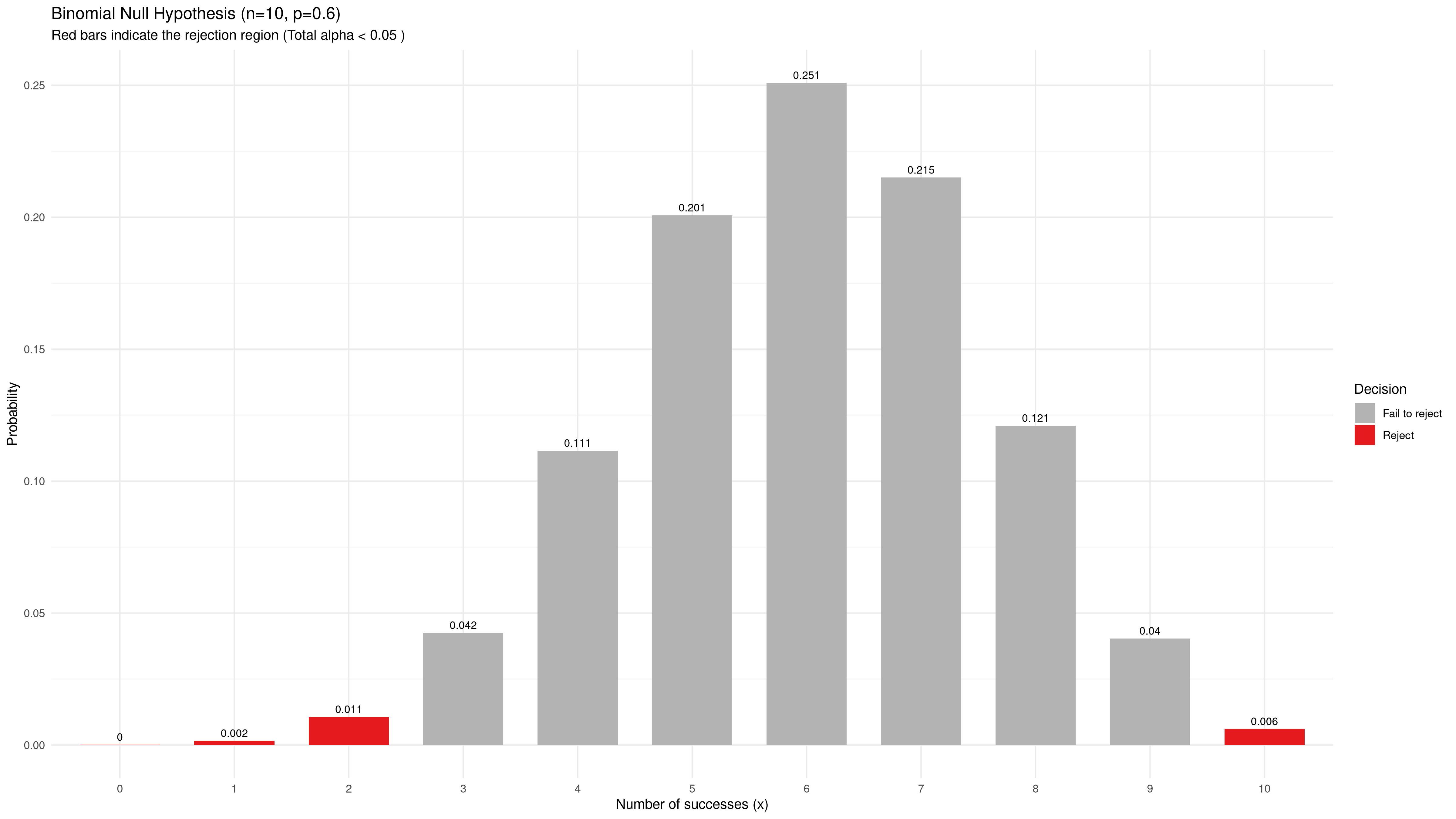
The probability of falsely rejecting the null hypothesis is about 2 %, somewhat less than our target $\alpha = 0.05$ due to the discrete distribution. Including one more bar on either side would bring us above that value.
Suppose the actual (but unknown) probability of winning with this new thing is 0.7 instead of the initial 0.6. That might be a small but useful improvement, about 0.2 standard deviations. The binomial distribution of wins among our 10 sample values is now like this:
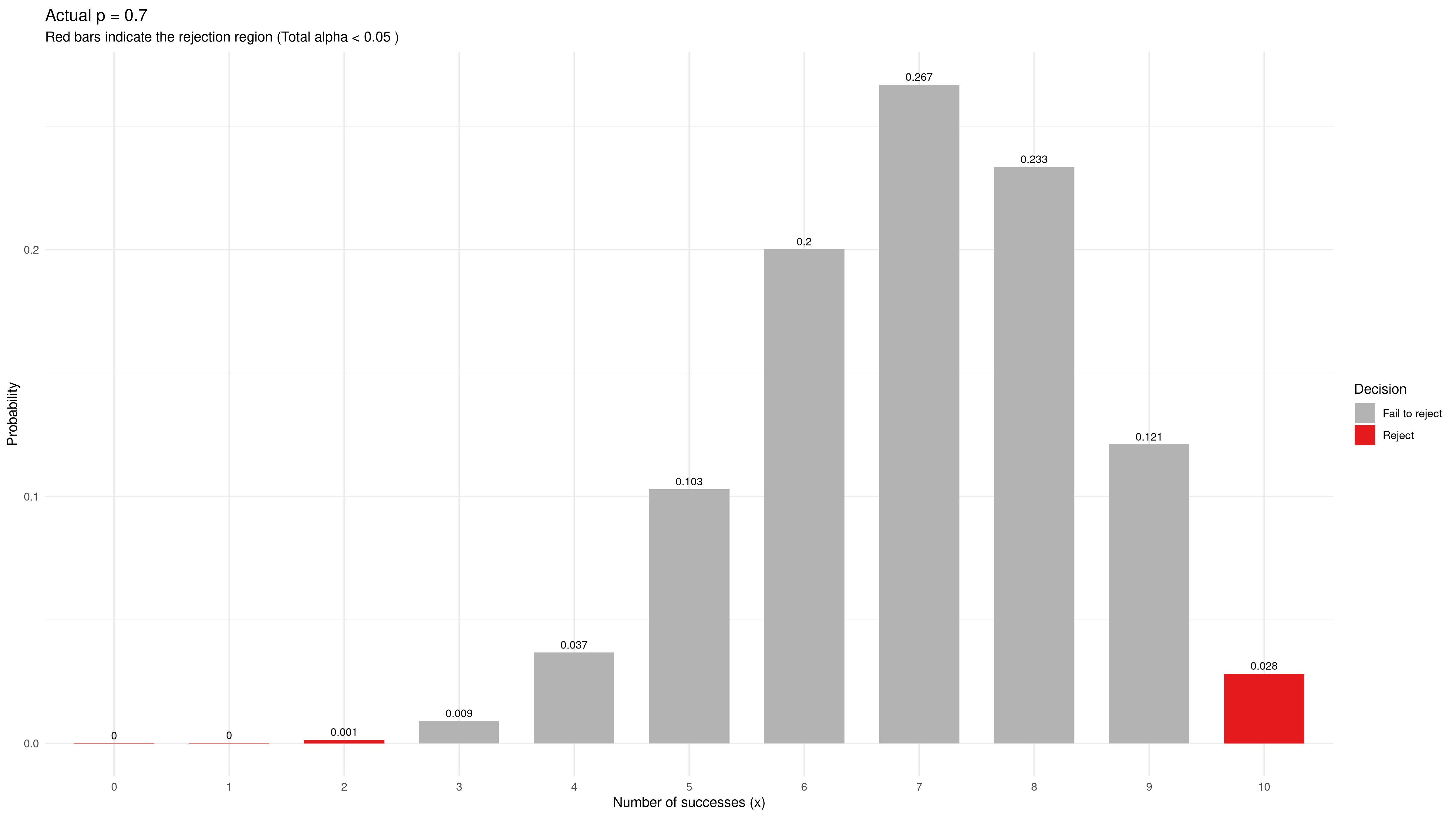
There is only about 3 % probability of rejecting the null hypothesis, and that includes a rather uncomfortable non-zero probability of concluding in the wrong direction from the actual effect.
Either way, our estimate of $p$ from a “statistically significant outcome” would wildly misjudge the actual effect size, such as $\hat{p} = 10/10 = 1.0$ or $\hat{p} = 2/10 = 0.2$ (or even worse). The proponents (or the detractors) would feel vindicated – “Look, that’s what I told you!” – but the result would not be anywhere near true.
We can plot the probability of rejecting the null hypothesis $p = 0.6$ as a function of the actual (unknown) success probability, as shown in the chart below. This is called a power curve, showing the experiment’s statistical power to resolve true differences from the null hypothesis.
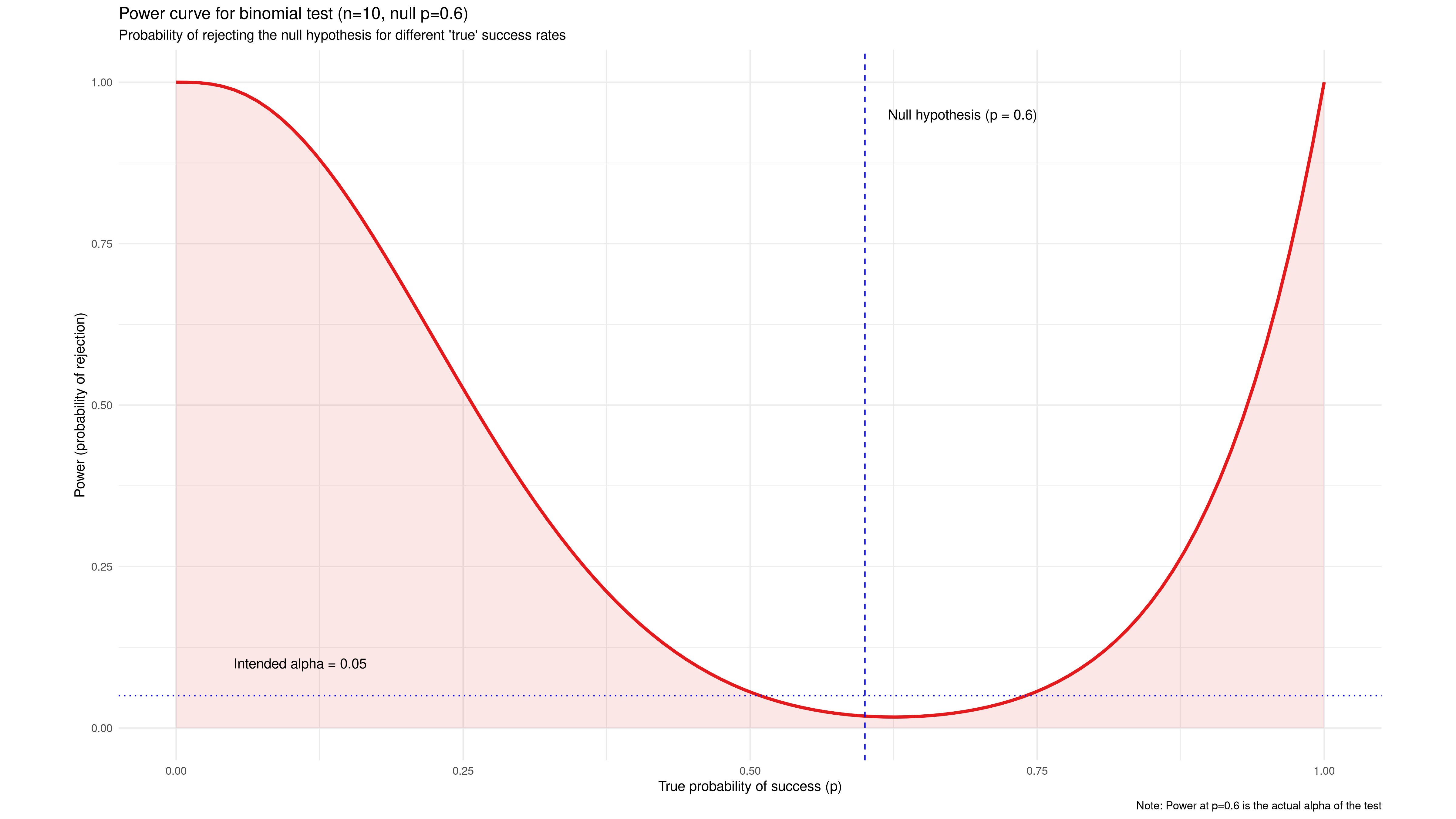
This one is seriously underpowered. Note that a wide area between $p = 0.5$ and $p = 0. 75$ has less probability of recognizing a real effect than our acceptable $\alpha = 0.05$. It is even asymmetric with the lowest probability for rejecting the null hypothesis at $p = 0.063$, slightly higher than the null hypothesis itself. Our test is virtually blind to small improvements, only able to reliably detect extreme values like $p < 0.1$ or $p > 0.95$.
But what if we could, say, implement our simulation model in a programming language that happened to run 45 times faster than this baseline, all else equal?
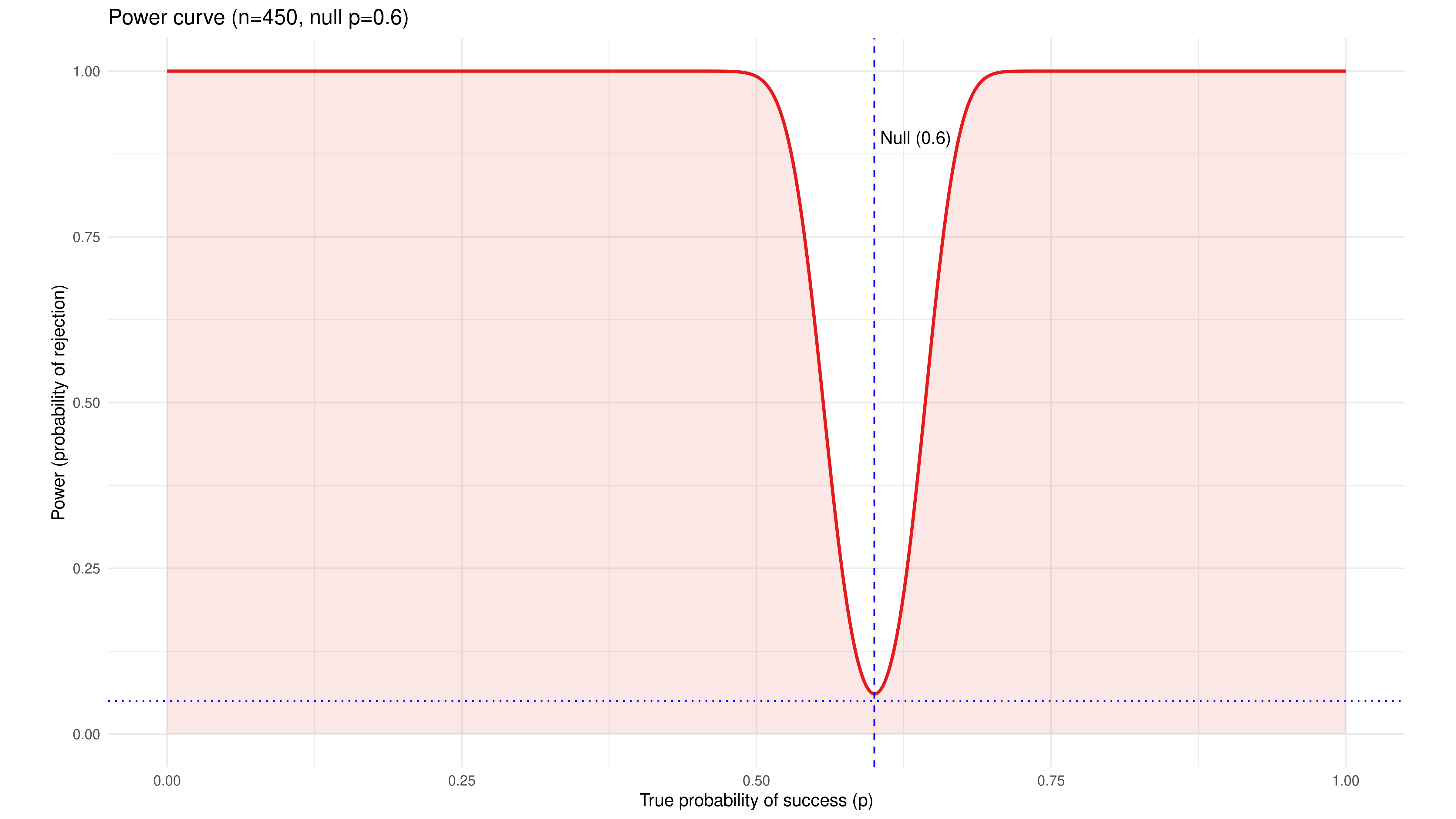
For the same budget of time and computing resources, we would then be able to run 450 replications instead of 10. Our power curve now turns into a precise notch filter, with a near-certain ability to detect any effect larger than 0.1 from our null hypothesis $p = 0.6$.
We can also plot the binomial test again for the null hypothesis $p = 0.6$, now with $n = 450$, and plot the sample distribution for an actual $p = 0.7$ in the same chart. This is a value just on the “shoulder” of the power curve. Almost the entire distribution of actual sample values now falls well outside the non-rejection region for our null hypothesis.
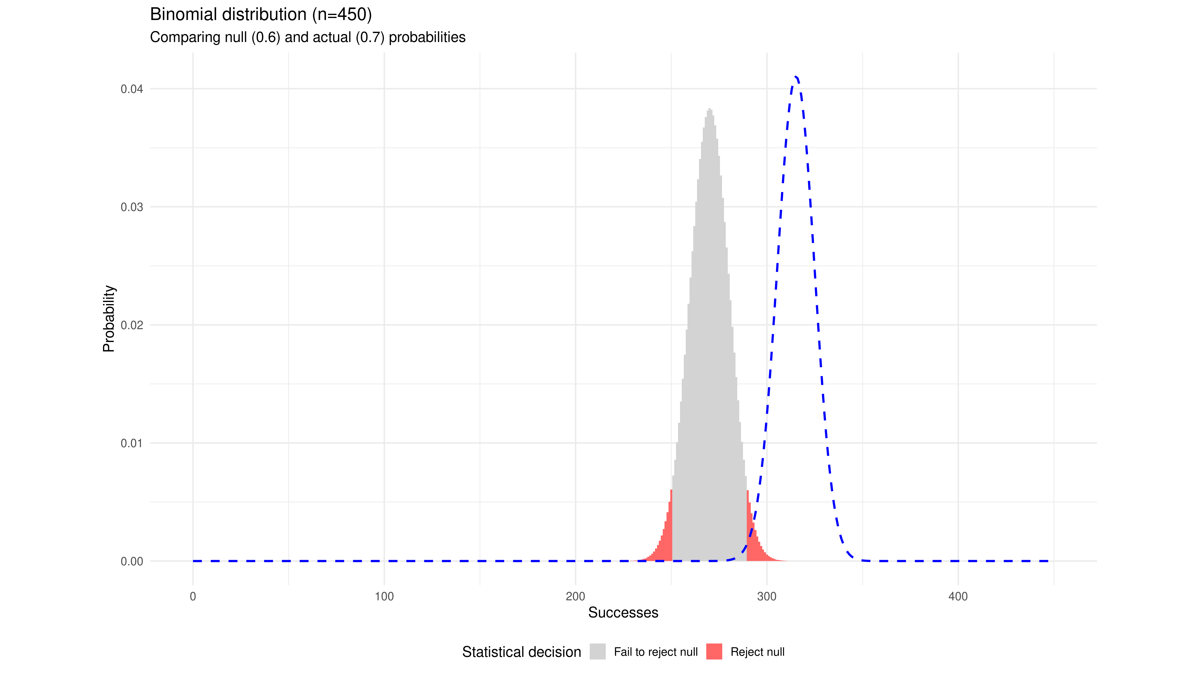
Our hypothetical 45x faster simulation has changed a blunt and opaque instrument into a high-powered magnifying glass. The improved speed translates directly into higher statistical power and higher analytical resolution.
This “hypothetical” 45x speed increase is the exact speed difference we have seen when benchmarking discrete event simulation models in C using the Cimba library against equivalent models in Python using SimPy and Python Multiprocessing. The increased statistical power follows from that.
One might argue that “Well, but we have so much more computing power now, so we can afford to be inefficient and slow.” I beg to differ. Analysts (and their clients) will always try to include more realistic model features up to a point where computing speed becomes a constraint. For example, in my models from around 1990, we modeled airborne sensor coverage as simple pie slices moving in two-dimensional airspace. What if one wanted higher realism, e.g., to model the dynamic three-dimensional sensor coverage from a maneuvering plane and the sensor cones from any approaching missiles, too? And perhaps replace my simple non-linear resource allocation model with something much more sophisticated for a more realistic representation of the human decision maker? Suddenly, the analyst is back to queueing for computer time in the time-honored fashion.
Speed is indeed (statistical) power.
One may also wonder how we actually were able to draw any conclusions at all back in the day, running such underpowered statistics on underpowered hardware.
The pragmatic approach could best be described as “informally Bayesian.” There was not enough power for proper frequentist hypothesis testing of each scenario, but over some time, we ran hundreds of simulations with various parameter values. That gave a keen sense of what was “typical” model output and what was most likely a statistical fluke. If something looked strange, we would run additional replications and variations around that point in the parameter space to try to understand what was going on. I believe we mostly got it right.
Leave a comment